Glioblastoma 1D PDE (Brain Tumor)

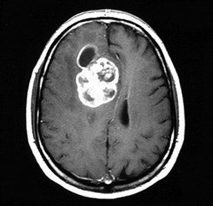
../_images/glioblastomaMRI.png — High-resolution MRI image of constrast-enhanced glioblastoma multiforme tumor. Adapted from J. S. Duncan, J. Tisi (2013)

This documentation describes the 1D Brain Tumor DPR (Diffusion-Proliferation-Radiation) Environment. The environment models the growth dynamics of glioblastomas–a fast-growing type of brain cancer–and their response to external beam radiation therapy (XRT). The model is governed by a partial differential equation (PDE) that includes three key terms: diffusion of tumor cells, proliferation, and radiation-induced cell death.

Background

Glioblastoma is the most common malignant primary brain tumor, accounting for approximately 16% of all primary brain tumors [1].

Glioblastomas are fast-growing and highly aggressive, with a median survival time of only 15 months following diagnosis [1]. Currently the standard treatment approach involves a combination of surgical resection (when possible), external beam radiation therapy (XRT), and concurrent chemotherapy. Magnetic Resonance Imaging (MRI) is used throughout treatment to monitor tumor progression and response to therapy.

Despite known differences in tumor growth across patients, clinical radiation therapy regimens remain largely standardized. This “one-size-fits-all” approach limits the ability to tailor treatment to individual tumors. Computational models such as the DPR framework aim to simulate tumor evolution under different protocols, offering a pathway toward more personalized therapy strategies.

One Dimensional Model

Although tumor growth occurs in three spatial dimensions and time, we make the assumption of a spherical tumor and that diffusion, proliferation, and radiation effects radially symmetric-dependent only on the distance from the tumor center. Under this symmetry assumption, the problem can be reduced to a one-dimensional formulation in the radial direction.

This reduction lets us simulate the 3D dynamics in a 1D spatial domain with far lower computational cost, while still capturing the tumor’s relevant growth and treatment behavior. The full nondimensionalization procedure and the derivation of the 1D model are described in detail in [2].

Let \(\mathcal{B} = [0, L]\) denote the one-dimensional spatial domain of the brain, where \(x=0\) corresponds to the tumor center and \(x=L\) is the outer boundary of the simulation domain. This domain models radial tumor expansion under the assumption of spherical symmetry.

Let \(\mathcal{T} = [0, T]\) denote the time domain of the simulation. Let \(\mathcal{T}_{\text{therapy}}\) represent the time intervals at which radiation therapy is administered. The tumor concentration \(c(x, t)\) evolves according to the following PDE:

\[\begin{split}\begin{aligned} c_t(x, t) &= \overbrace{D\nabla^2 c}^{\text{diffusion}} + \overbrace{\rho c (1 - c/K)}^{\text{proliferation}} - \overbrace{R(\alpha, \beta, d(x, t), t) c (1 - c/K)}^{\text{radiation}}, && (x, t) &\in \mathcal{B} \times \mathcal{T} \\ c(x, 0) &= 0.8 K e^{-0.25x^2}, && x &\in \mathcal{B} \\ \mathbf{n} \cdot \nabla c(x, t) &= 0, && (x, t) &\in \partial \mathcal{B} \times \mathcal{T} \end{aligned}\end{split}\]

where a zero-flux (Neumann) boundary condition is imposed at the spatial boundaries to ensure that no tumor cells enter or leave the domain during the simulation. \(\nabla c\) is the spatial gradient of the tumor concentration and \(\mathbf{n}\) is the outward-pointing unit normal vector at the boundary \(\partial \mathcal{B}\) of the spatial domain.

The radiation term \(R\) is given by:

\[\begin{split}\begin{aligned} R(\alpha, \beta, d(x, t), t) &= \begin{cases} 1 - S(\alpha, \beta, d(x, t)), & \text{if } t \in \mathcal{T}_{\text{therapy}} \\ 0, & \text{otherwise} \end{cases} \\ S(\alpha, \beta, d(x, t)) &= e^{-\alpha \cdot \gamma(\alpha, \beta, d(x, t))} \\ \gamma(\alpha, \beta, d(x, t)) &= \varphi \cdot d(x, t) \left( 1 + \frac{d(x, t)}{\alpha / \beta} \right) \end{aligned}\end{split}\]

where we provide the physical interpretation of all the environment variables below:

\(D\): diffusion coefficient in units \((mm^2/day)\)
\(\rho\): proliferation rate in units \((1/day)\)
\(K\): carrying capacity, maximum supported cell density, in units \((cells/mm^3)\)
\(\varphi\): fractions per day (FPD). Describes how many parts each treatment day’s dose is split into.
\(d(x, t)\): fractionated radiation dose in Gray \((Gy = J/kg)\) applied at spatial location \(x\) and time \(t\). This value represents 1 of \(\varphi\) dose fractions delivered at each treatment instance (\(\varphi \cdot d(x, t) =\) total dosage given in 1 day of treatment). Dose distribution varies spatially depending on the tumor’s size, and temporally based on treatment schedule
\(\alpha\): radio-sensitivity parameter in \((Gy^{-1})\) that qualifies probability of immediate (single-hit) cell death caused by radiation. In the linear-quadratic model for radiation efficacy, this term governs the linear component of damage
\(\beta\): radio-sensitivity parameter in \((Gy^{-2})\) that qualifies probability of quadratic (double-hit) cell death, where two radiation-induced sub-lethal damages combine to cause cell death. In the linear-quadratic model for radiation efficacy, this term governs the quadratic component of damage
The function \(\gamma(\cdot)\) represents the biologically effective dose (BED) which scales the efficacy of radiation treatment by number of fractions given by \(\varphi\), and \(\alpha\) and \(\beta\)
The function \(S(\cdot)\) represents the probability a tumor cell survives given that it received radiation dose \(d\)
The function \(R(\cdot)\) represents the probability a tumor cell dies given that it received radiation dose \(d\)

Radiation Therapy Schedule

The external beam radiation therapy schedule follows a slightly modified version of the standard protocol adopted by the University of Washington Medical Center [2]. In our environment, the schedule spans 34 treatment days of 1.8 \((Gy)\) each, delivered to the T2 region + a 25 mm margin for a total of 61.2 \((Gy)\). The environment supports both continuous treatment delivery over 34 consecutive days and a clinically realistic 5-days-on, 2-days-off schedule to account for weekend breaks.

Environment Implementation Details

Our environment is built on mathematical modeling approaches developed in [2], [3], and [4], which are widely adopted in the glioblastoma modeling literature.

Simulated MRI Scans

Glioblastoma diagnosis and treatment monitoring are typically performed using two types of MRI scans: gadolinium enhanced T1-weighted and T2-weighted imaging (referred to here as T1 and T2, respectively). While these scans do not directly measure tumor cell density, prior modeling studies have established heuristic thresholds that map simulated tumor density to visible MRI regions [5]:

The T1 region corresponds to areas of high tumor cell density, typically >80% of the carrying capacity
The T2 region corresponds to areas of moderate tumor cell density, typically >16% of the carrying capacity

Although our model explicitly evolves only the tumor cell density \(c\), these thresholds allow us to generate synthetic MRI images. By interpreting the density distribution at each timestep, we simulate the clinical appearance of T1 and T2 scans and track tumor radii dynamically over time. This also enables us to spatially define the radiation dose function \(d(x,t)\) in accordance with evolving tumor boundaries during therapy.

Simulation Details

The simulation state \(c\) is modeled as a two-dimensional array of shape \((nt, nx)\), where each entry represents the tumor cell density at a specific time step and spatial position. The governing PDE is solved using an explicit finite-difference scheme.

The simulation proceeds through 3 sequential stages:

Growth Stage: Beginning from the initial condition, the tumor undergoes unconstrained proliferation until the T1 detection radius of 15mm is reached. This marks the onset of the therapy stage.
Therapy Stage: The radiation therapy schedule described above is applied. On each treatment day, the dose distribution \(d(x, t)\) is recalculated based on the current T2 radius, determining the spatial region receiving radiation.
Post-Therapy Stage: After completion of therapy, the tumor continues to grow freely until the T1 death radius of 35mm is reached or the simulation reaches its final temporal step.

Parameters (taken from [4])

\(D\) = 0.2 \((mm^2/day)\)
\(\rho\) = 0.03 \((1/day)\)
\(K\) = \(10^5 (cells/mm^3)\)
\(\varphi\) = 1
\(\alpha\) = 0.04 \((Gy^{-1})\)
\(\alpha / \beta\) = 10 \((Gy)\)
T1 detection radius = 15 \((mm)\)
T1 death radius = 35 \((mm)\)
Total treatment dosage = 61.2 \((Gy)\)

Reinforcement Learning Framework

RL Formulation

The radiation therapy schedule described above represents a one-size-fits-all approach applied uniformly across patients, despite individual differences in tumor growth characteristics and radiation sensitivity (driven by varying diffusion coefficients, proliferation rates, and radio-sensitivity constants).

In our framework, we focus on the therapy stage and model it as a reinforcement learning problem. Here, the tumor state \(c\) is exposed as the observation space, and the RL agent determines the action–how much radiation dosage to apply–at each treatment step.

A hard constraint enforces the total allowable radiation dose, whose depletion marks the end of therapy. A soft constraint, derived from the clinically safe dosage for a given treatment radius, penalizes excessive dosage that may risk patient safety. The function dmaxsafe(treatmentRadius) defining the safe dosage for a given treatment radius is extrapolated from clinical data in [6].

Our custom reward function encodes both treatment efficacy and safety to guide the RL agent toward an optimal, patient-specific therapy schedule.

Reward Function

The reward function, which the RL agent seeks to maximize, consists of two components: a large episodic reward and possibly negative step reward.

\[\begin{split}\begin{aligned} R_{episode}(t) &= t - t_{benchmark},\quad \text{if } t \in deathday \\ R_{step}(TR,AD,TD) &= \begin{cases} 0, & \text{if } AD \le dmaxsafe(TR) \\ -\lambda\!\left(\dfrac{AD-dmaxsafe(TR)}{TD-dmaxsafe(TR)}\right)^{1/3}, & \text{if } AD \gt dmaxsafe(TR) \end{cases} \end{aligned}\end{split}\]

where:

\(TR\) - treatment radius in units \((mm)\)
\(AD\) - applied dose in units \((Gy)\)
\(TD\) - total dose in units \((Gy)\)

The episodic reward corresponds to the number of additional days the patient survives compared to a benchmark simulation with no treatment.

The step reward introduces a soft safety constraint, penalizing dosage values that exceed the safe clinical threshold. The cubic root ensures a smooth but stepp increase in penalty for even small violations.

The agent’s objective is therefore to maximize total reward by extending survival while minimizing (ideally eliminating) violations of the safety constraint.

Training Details

We train a PPO agent on this environment. The agent interacts only during the therapy stage, observing the current tumor state \(c\) and choosing a continuous action \(a \in [0, 1]\), the proportion of total dosage to apply at the current timestep. If the proposed dosage exceeds the remaining allowed dose or meets a termination threshold, the environment automatically applies the remaining dosage and transitions to the post-therapy stage. A wrapper class is used to encapsulate the growth and post-therapy stages, simulating them internally so that they remain invisible to the PPO agent.

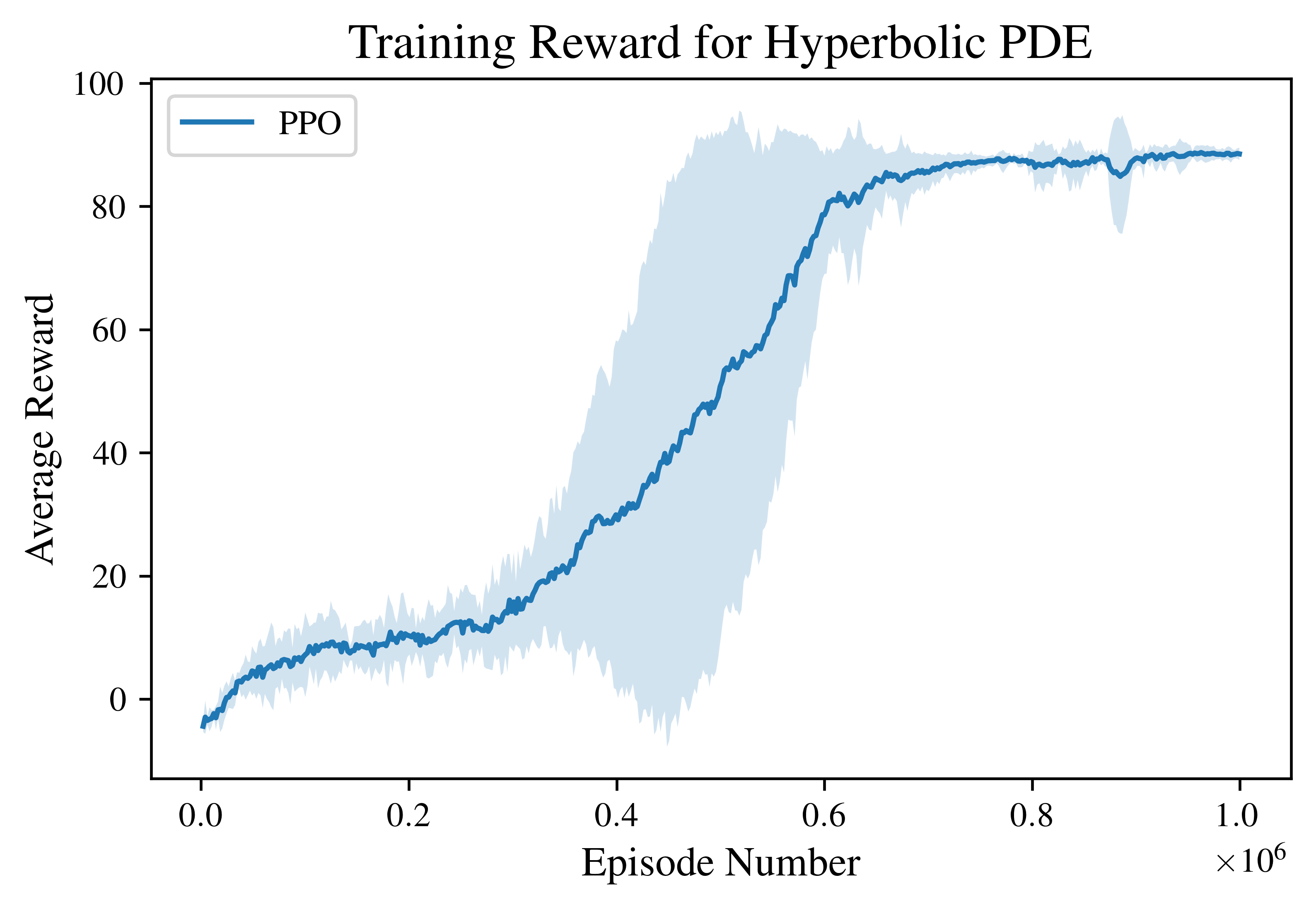
For all experiments, we train the PPO agent for a total of \(10^6\) environment steps.

The graph below shows the resulting train reward curve. The solid line indicates the mean episodic reward over 4 independent training runs, while the shaded region represents the 95% confidence interval. The agent rapidly improves after approximately \(3\times10^5\) steps, and converges to a stable high-reward policy by the end of training.

Results and Analysis

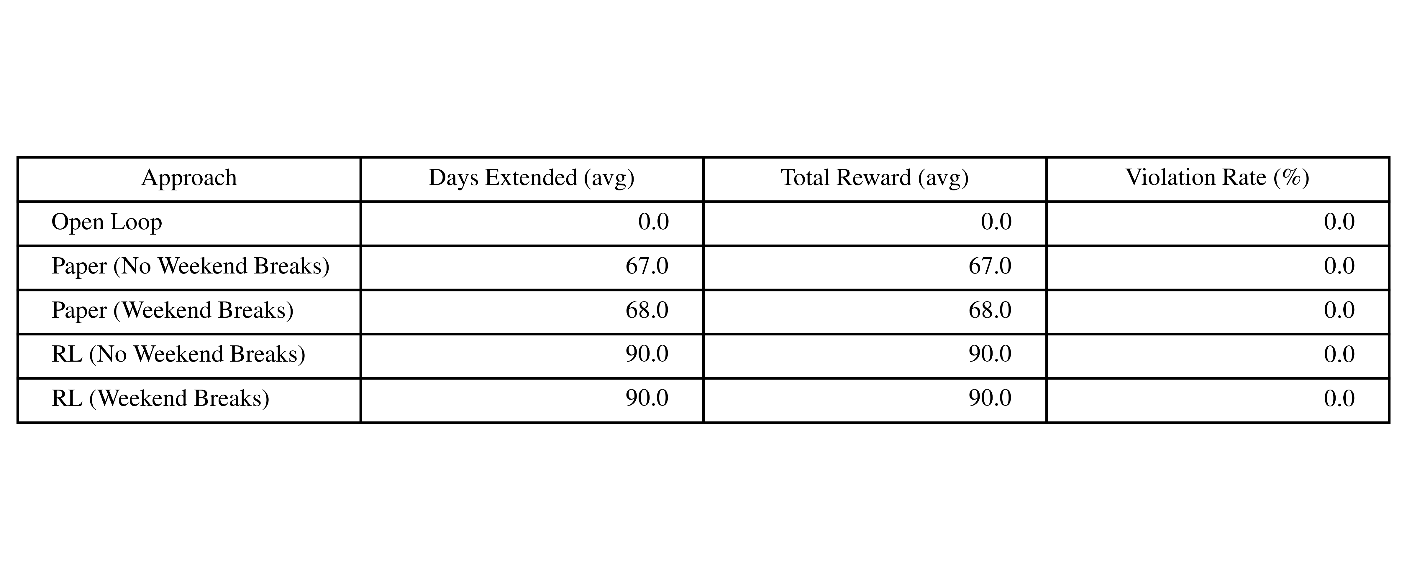
We compare the RL policy against three baselines:

Open Loop (No Control) - zero radiation dosage given
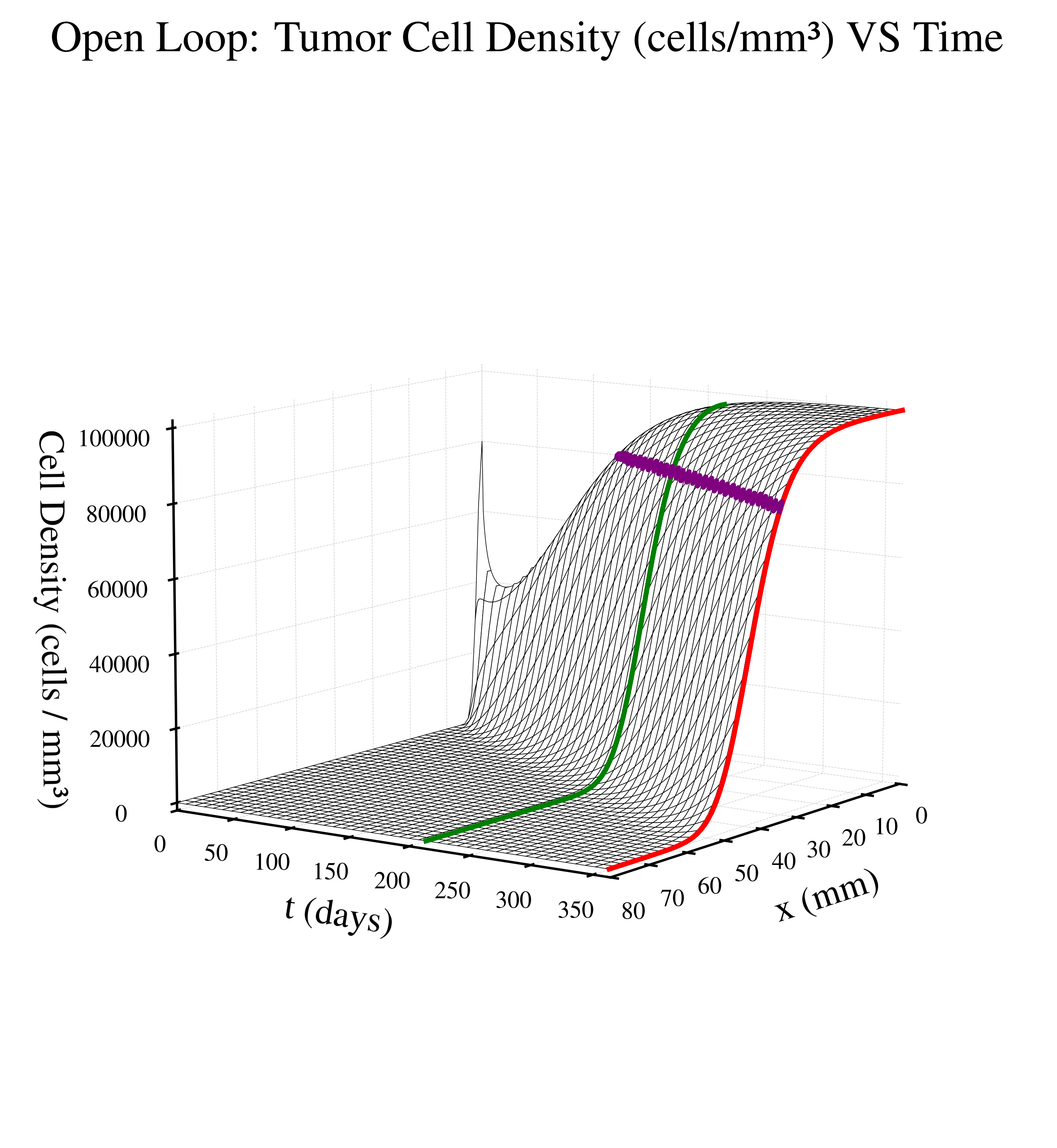
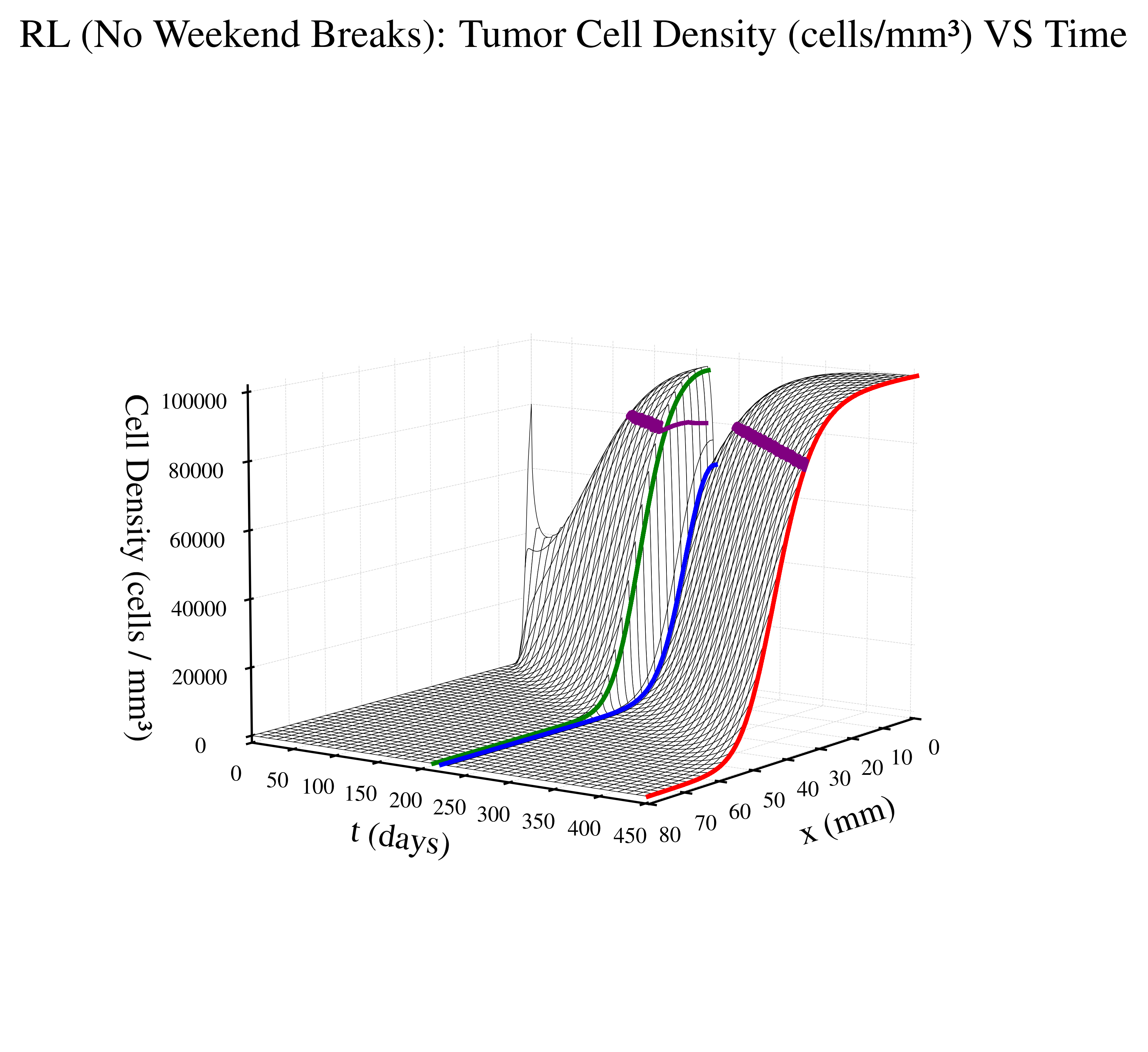
Paper Protocol (No Weekend Breaks) - based on the above defined radiation therapy schedule where patient gets no weekend breaks
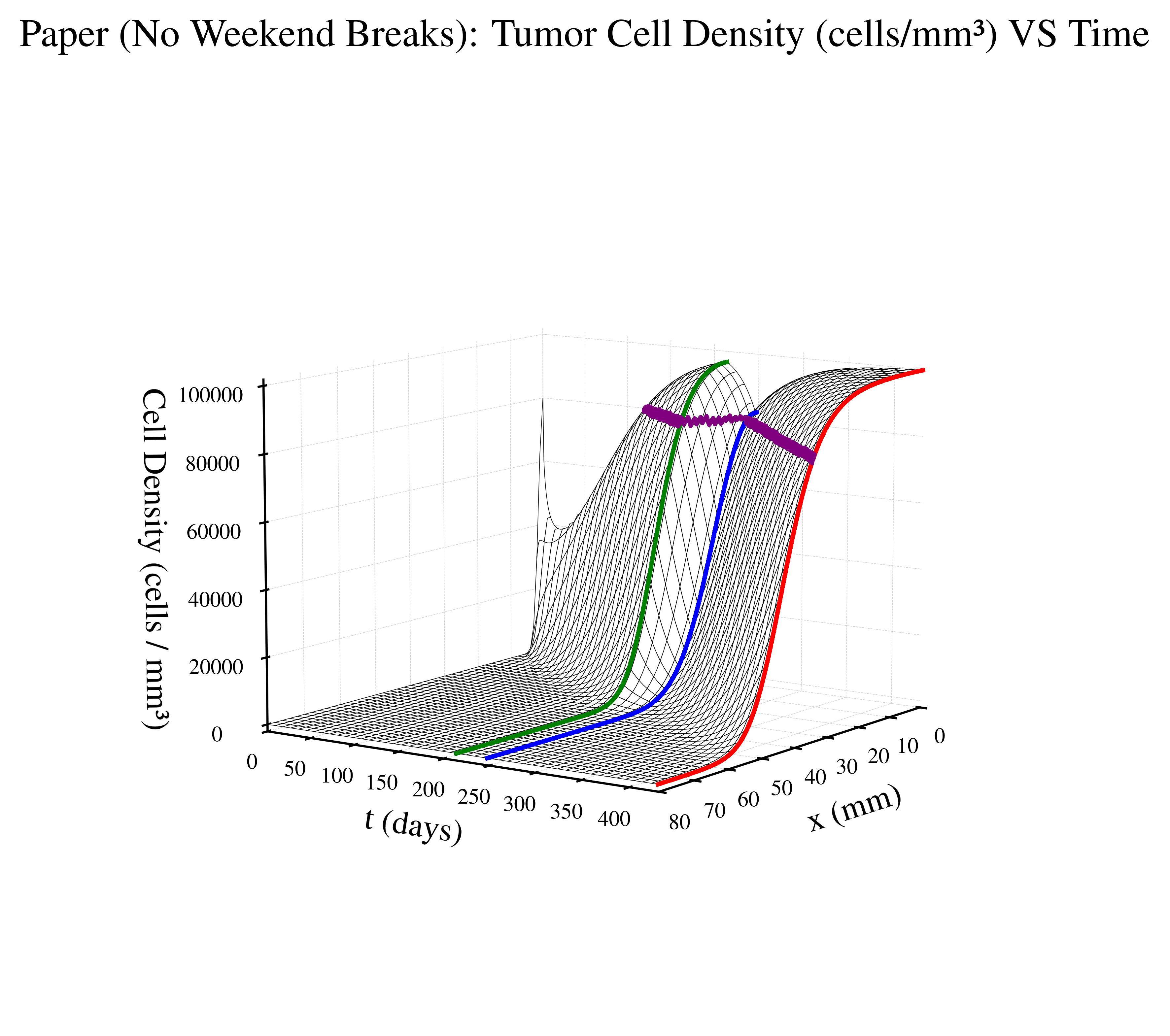
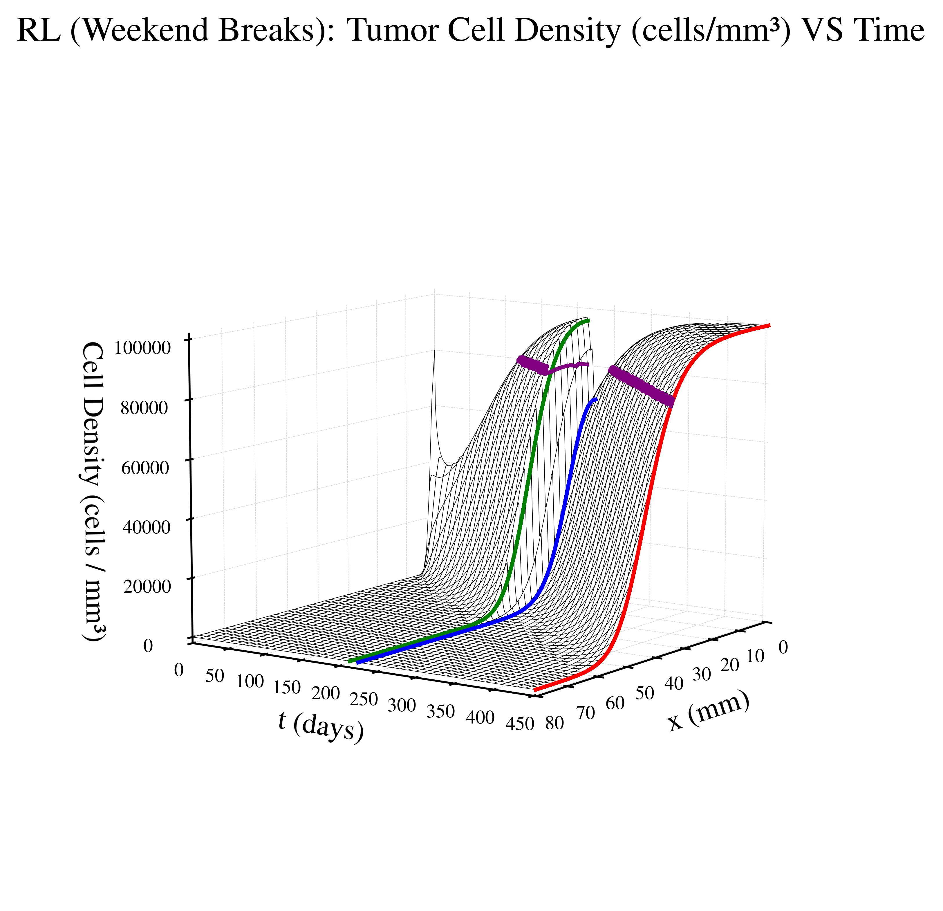
Paper Protocol (Weekend Breaks) - based on the above defined radiation therapy schedule where patient gets weekend breaks

Below is a table summarizing results for each approach. For each approach, we run five simulation episiodes and average days lived, total reward, and the violation rate. Violation rate is defined as proportion of total therapy steps where our soft constraint is violated, that is, when our applied radiation dose is greater than dmaxsafe(treatmentRadius) allows.

What the table shows is that our RL-based schedule extends patient survival by over 20 days compared to traditional protocols while maintaining complicance with the soft safety constraint.

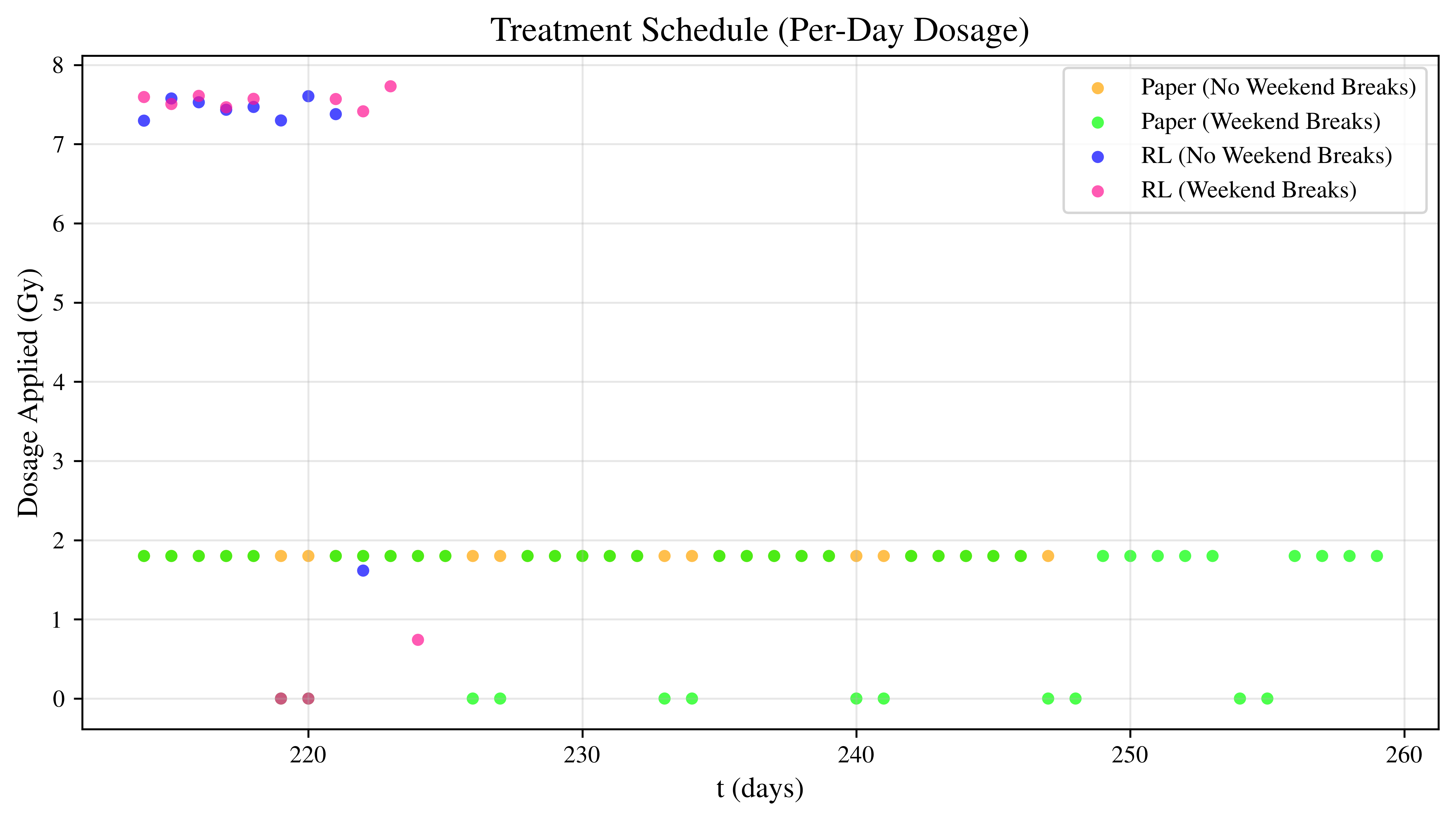
The corresponding treatment schedules for a representative episode are shown below. Dose in Gy is plotted against given treatment day:

The figures below visualize the internal tumor state (cell density over time and space) for a representative episode of treatment approach. The time domain for each graph depends on patient survival time.

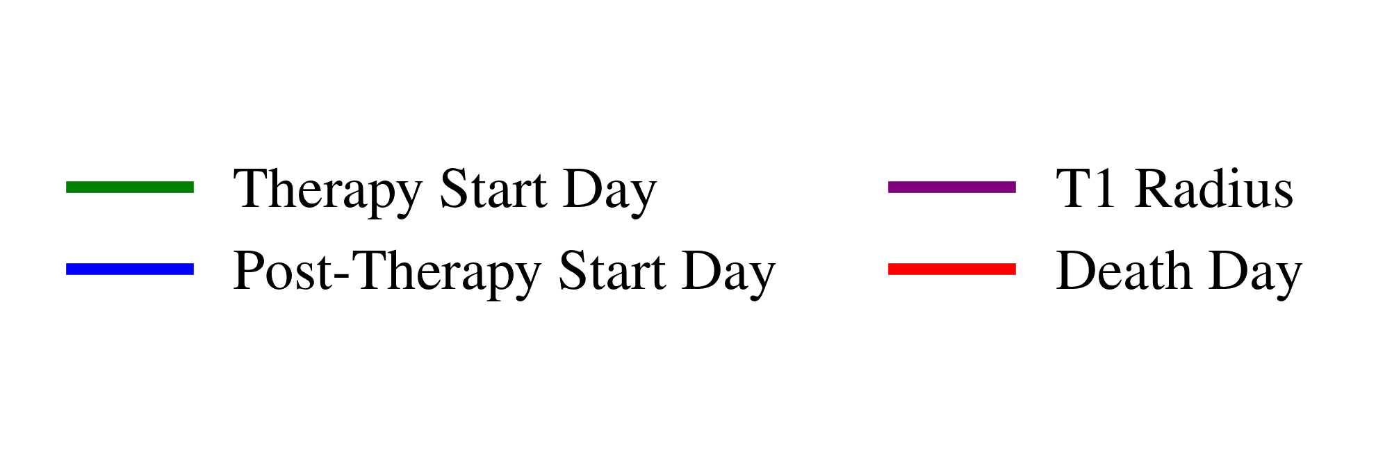
Numerical Implementation

We derive the numerical implementation scheme for those looking for inner details of the environment. We use a first-order finite-difference scheme to approxiate the dimensionless PDE:

\[c_t(x, t) = D\nabla^2 c + \rho c (1 - c/K) - R(\alpha, \beta, d(x, t), t) c (1 - c/K)\]

Consider the first-order taylor approximation as

\[c(x, t+1) = c(x, t) + \Delta t \cdot c_t(x, t)\]

with finite spatial derivatives approximated by first-order centered differences where \(c_{j}^{n}\) is shorthand for \(c(x_{j}, t_{n})\)

\[\frac{\partial^2 c}{\partial x^2} = \frac{c_{j+1}^n - 2c_j^n + c_{j-1}^n}{(\Delta x)^2}\]

where \(\Delta t = dt = \text{time step}\), \(\Delta x= dx = \text{spatial step}\), \(n=0, ..., Nt\), \(j=0, ..., Nx\), where \(Nt\) and \(Nx\) are the total number of discretized temporal and spatial steps respectively. Substituting into our original equation yields

\[c_{j}^{n+1} = c_{j}^{n} + \Delta t (D \cdot (\frac{c_{j+1}^n - 2c_j^n + c_{j-1}^n}{(\Delta x)^2}) + \rho c_{j}^n (1 - c_{j}^n/K) - R(\alpha, \beta, d(x,t), t) c_{j}^n (1 - c_{j}^n/K))\]

The last thing to consider is the boundary conditions for finding \(c_{j}^{n+1}\) when \(j = 0\) or \(j = Nx\). In these cases, we set \(c_{0}^{n} = c_{1}^{n}\) and \(c_{Nx}^{n} = c_{Nx-1}^{n}\) respectively to create a symmetric and mirrored concentration field across the boundary to satisfy the no-flux boundary condition.

API Reference

This section provides detailed documentation of the Python classes, methods, and utilities implementing the Glioblastoma 1D PDE environment and reinforcement learning interface.

See the Utilies -> Pre-implemented Rewards section for the API reference for the environment’s corresponding reward class.