1D Traffic ARZ PDE Tutorial
This tutorial will follow the Jupyer-notebooks found at github. We will explore the Traffic Aw–Rascle–Zhang (ARZ) PDE environment, which consists of 1D coupled hyperbolic PDEs that models traffic flow on freeways. The contontrol objective is to stabilize the traffic flow to a desired steady state traffic density and velocity.
We first start by initializing the TrafficARZ1D environment. The environment is initialized with the following parameters:
T = 240
dt = 0.25
dx = 10
X = 500

from pde_control_gym.src import TrafficARZReward
reward_class =  TrafficARZReward()

Parameters = {
        "T": T,
        "dt": dt,
        "X": X,
        "dx": dx,
        "reward_class": reward_class,
        "simulation_type" : 'inlet',
        "v_steady" : 10,
        "ro_steady" : 0.12,
        "v_max" : 40,
        "ro_max" : 0.16,
        "tau" : 60
}
Detailed explanation about the parameters can be found in the TrafficARZ1D environment documentation. A short description of the parameters we have initialized is as follows:
T: Total simulation time in seconds.dt: Time step in seconds.X: Length of the road in meters.dx: Spatial step in meters.reward_class: The reward class to be used for the environment. In this case, we use theTrafficARZRewardclass.simulation_type: The type of simulation to be run. In this case, we use theinletsimulation type, which means that the traffic flow is controlled at the inlet of the road.v_steady: The desired steady state velocity of the traffic flow in meters/second.ro_steady: The desired steady state traffic density in vehicles/meter.v_max: The maximum velocity of the traffic flow in meters/second permissible on freeway.ro_max: The maximum traffic density in vehicles/meter permissible on freeway.tau: The time taken by drivers to adjust to new traffic conditions in seconds.
We can now instantiate the trafficARZ environment as follows:
from pde_control_gym.src.environments import TrafficARZ1D
envBcks = gym.make("PDEControlGym-TrafficPDE1D",**Parameters)
Before, building the controller model, we need to define a function that sequentially applies the control actions to the environment. This function will be used to run a simulation episode and store the data obtained from each timestep for further analysis. The function will take a model (controller) and an environment as input, and it will return the cumulative reward, the environment state history, the action history, and the reward history as follows:
def runSingleEpisode(model, env, parameter = None):
    terminate = False
    truncate = False

    # Holds the resulting states
    uStorage = []

    # Reset Environment
    obs,__ = env.reset()
    uStorage.append(obs)

    ns = 0
    i = 0

    #Cummulative reward
    rew = 0

    #Storing action and reward history
    act_h = []
    rew_h = []

    while not truncate and not terminate:
        action = model(env,obs,parameter)
        act_h.append(action)
        obs, rewards, terminate, truncate, info = env.step(action)
        uStorage.append(obs)
        rew += rewards
        rew_h.append(rewards)
        ns += 1
    u = np.array(uStorage)
    return rew, u, act_h, rew_h
PDE Backstepping Controller
Let \(\rho(x,t)\), \(v(x,t)\) and \(q(x,t)\) represent the traffic density, velocity, and traffic flux respectively and the control objective is to stabilze the values of these parameters around \(\rho^\star\), \(v^\star\), and \(q^\star\) respectively. The detailed explanations of the notations can be found in TrafficARZ1D environment documentation. The PDE backstepping controller is designed to achieve this control objective by applying a control input \(q(x=0, t)\) and \(q(x=L, t)\) at the boundaries of the freeway.
The inlet backsteeping controller is given by the following equation:
The kernels for outlet backsteeping controller are given by:
where \(\gamma\) is a scaling factor and \(p^\star = \frac{v_{max} r^\star}{r_{max}}\). We now define the following characteristic speeds of the backstepping controller:
The spatial feedback weights are given by:
Then the outlet boundary control input is given by:
\begin{align} q(x = L, t) = q^\star + \rho^\star \int_0^L c_v(x) (v(x) - v^\star) \, dx + \int_0^L c_q(x) (q(x) - q^\star) \, dx \end{align}
The below code implements the above equations to create a backstepping controller for the inlet and outlet control scenarios.
def bcksController(env, obs, parameter=None):
    if env.unwrapped.simulation_type == 'inlet':
        #Inlet control
        return env.unwrapped.qs

    elif env.unwrapped.simulation_type == 'outlet' or env.unwrapped.simulation_type == 'both':
        #Outlet control
        x = np.arange(0, env.unwrapped.L + env.unwrapped.dx, env.unwrapped.dx)
        lambda1 = env.unwrapped.vs
        lambda2 = env.unwrapped.vs + env.unwrapped.rs * (-env.unwrapped.vm / env.unwrapped.rm)

        gamma = 1
        K_kernel = -(1 / (gamma * env.unwrapped.ps)) * (-1 / env.unwrapped.tau) * np.exp(-x / (env.unwrapped.tau * env.unwrapped.vs))
        M_kernel = - K_kernel

        cv = M_kernel + (lambda2 / lambda1) * K_kernel * np.exp(x / (env.unwrapped.vs * env.unwrapped.tau))
        cq = ((lambda1 - lambda2) / lambda1) * K_kernel * np.exp(x / (env.unwrapped.vs * env.unwrapped.tau))

        v = env.unwrapped.v
        q = env.unwrapped.r * env.unwrapped.v
        v_err = v - env.unwrapped.vs
        q_err = q - env.unwrapped.qs

        integral_v = np.trapz(cv.flatten() * v_err.flatten(), dx=env.unwrapped.dx)
        integral_q = np.trapz(cq.flatten() * q_err.flatten(), dx=env.unwrapped.dx)

        q_out = env.unwrapped.qs + env.unwrapped.rs * integral_v + integral_q

        if env.unwrapped.simulation_type == 'outlet':
            return q_out
        else:
            return (env.unwrapped.qs,q_out)
The below command will run the simulation episode using the backstepping controller we have defined above:
rew, u, act_h, rew_h = runSingleEpisode(bcksController, envBcks, None)
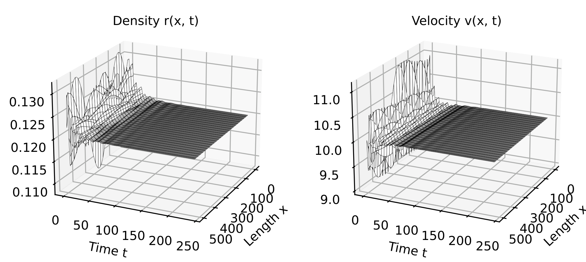
The trajectory obtained after backstepping control for simultaneous inlet and outlet control is shown below. It can be observed that the traffic density and velocity converge to the desired steady state values.
Reinforcement Learning Controller
The Reinforcement Learning (RL) controller uses Proximal Policy Optimization (PPO) to stabilize traffic flow by controlling boundary conditions. This approach learns optimal control policies through interactions with the environment. We start by intializing the gym for training.
T = 240
dt = 0.25
dx = 10
X = 500

from pde_control_gym.src import TrafficARZReward
reward_class =  TrafficARZReward()

Parameters = {
        "T": T,
        "dt": dt,
        "X": X,
        "dx": dx,
        "reward_class": reward_class,
        "simulation_type" : 'outlet-train',
        "v_steady" : 10,
        "ro_steady" : 0.12,
        "v_max" : 40,
        "ro_max" : 0.16,
        "tau" : 60,
        "limit_pde_state_size" : True,
        "control_freq" : 2
}
Here, the limit_pde_state_size parameter is set to True to limit the size of the PDE state space to ensure numerical stability while traning. The control_freq parameter is set to 2, which means the control input is applied every two PDE simulation steps using a zero-order hold approach, effectively holding the control constant while the PDE evolves between updates. This allows the RL model more time to learn the optimal control action.
Then, we deaclare some callbacks to log the training metrics to TensorBoard and to save the model checkpoints during training.
#Declaring required callbacks for checkpointing and logging
checkpoint_callback = CheckpointCallback(
save_freq=50000,
save_path="./logsPPO",
name_prefix="rl_model",
save_replay_buffer=True,
save_vecnormalize=True,
)

class RewardLoggingCallback(BaseCallback):
    def __init__(self, verbose=0):
        super(RewardLoggingCallback, self).__init__(verbose)

    def _on_step(self):
        # Log the rewards at each step to TensorBoard
        self.logger.record('reward', np.mean(self.locals['rewards']))
        return True
reward_logging_callback = RewardLoggingCallback()
callback_list = CallbackList([checkpoint_callback,reward_logging_callback])
The traning of the PPO policy is done using Stable Baselines3 library for 2,000,000 timesteps as follows:
Parameters["simulation_type"] = 'outlet-train'
envRL = gym.make("PDEControlGym-TrafficPDE1D",**Parameters)

model = PPO("MlpPolicy",envRL, verbose=1, tensorboard_log="./tb/")

#Training the model (Trained models are avaiable in our HuggingFace repo)
model.learn(total_timesteps=2000000, callback=callback_list)
The trained model is available in our HuggingFace repository at PDEControlGymModels. These models can be directly used to run the simulation episodes without running the above training code.
Now, we define a RL controller function that uses the trained PPO model to control the traffic flow. The function takes the environment, previous timestep observation and the trained model as input and returns the control action:
def RLController(env,obs,model):

    #Normalization of observation space
    half = obs.shape[0] // 2
    r = obs[:half]
    v = obs[half:]
    obs_sc = np.reshape(
        np.concatenate(((r - env.unwrapped.rs) / env.unwrapped.rs, (v - env.unwrapped.vs) / env.unwrapped.vs)),
        -1
    )

    #Predicting action using RL model
    action, _state = model.predict(obs_sc)

    if env.unwrapped.simulation_type == 'outlet':
        return action[0]
    elif env.unwrapped.simulation_type == 'both':
        return (env.unwrapped.qs, action[0])
Note that the PPO algorithm performs better with normalized observation space and the same is used while training the model. So, the action prediction should also be done using the normalized observation space.
Finally, the simulation episode can be run using the trained RL controller as follows:
Parameters["simulation_type"] = 'both'
Parameters["control_freq"] = 1
PPO_model = PPO.load('./logsPPO/rl_model_1500000_steps.zip')
env = gym.make("PDEControlGym-TrafficPDE1D",**Parameters)
rew, u, act_h, rew_h = runSingleEpisode(RLController, env, PPO_model)
Here, the control_freq to 1 to simulate the PDE once per action.
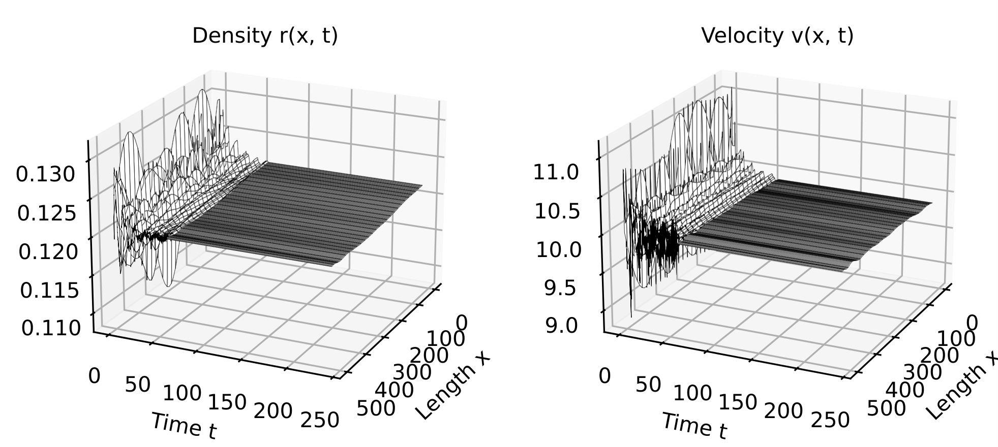
The trajectory obtained after RL control for simultaneous inlet and outlet control is shown below. Again, it can be observed that the traffic density and velocity converge to the desired steady state values.
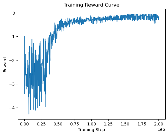
The reward curve obtained during RL training is shown below. We can observe that it begins with low values and gradually increases, eventually saturating as the model learns to stabilize traffic flow.